Let’s say you are running a business. You have just on-boarded an (expensive) new agency for acquiring customers. After a month, you want to decide if you should continue using them. You do this by comparing the average revenue of customers brought in by them agency, to average revenue of customers from your existing channels. How many customers from that agency do you need, to make an informed decision? 10? 50? 500?
Per-customer revenue is usually very long tailed. This means a small number of customers contribute a large part of the revenue. Most people lack statistical intuition for long tailed distributions and grossly underestimate the number of customers required to make a data-driven decision. With 50 customers, your estimate could still easily be off a factor of \(\frac{1}{2}\) to \(2\).
To make matters worse: With a small number of customers in your sample, you’re likely to underestimate the true average. This would make the new agency look worse than it actually is. Not considering this, you might set yourself up to make systematically sub-optimal decisions.
We’ll take a closer look at why, and what you can do, using very little math.
Per-customer revenue is usually long tailed
If you’re running a transaction-based business, the distribution of revenue brought by each customer during their early lifetime probably looks something like this:
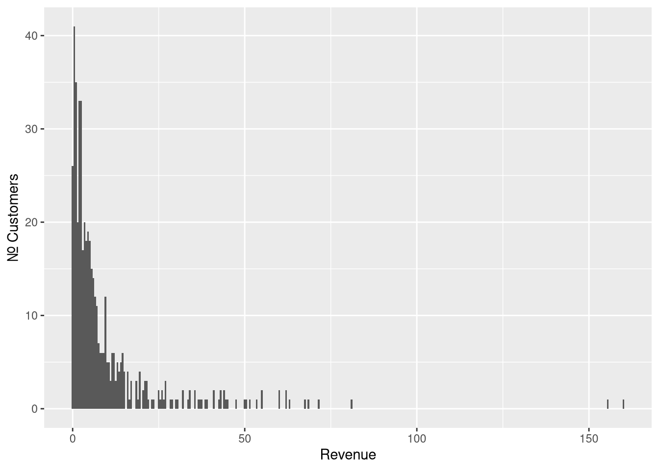
Figure 1: Samples from Pareto Type II distribution with scale=10, shape=2 and location=0
This may be all familiar: A large number of customers are in the low range. Only a few customers are in the high range (the long tail), but they contribute a disproportionately large amount to your total revenue. This is often referred to as the 80/20-rule, or the Pareto principle.
Sampling from long tailed distributions
This long tail of the distribution is a problem when trying to estimate average revenue. Customers in the tail are frequent enough to have a considerable impact on the average. At the same time, they are rare enough to make it difficult to estimate how frequent they actually are.
To build intuition for this, let’s uniformly sub-sample 5% of the original sample:
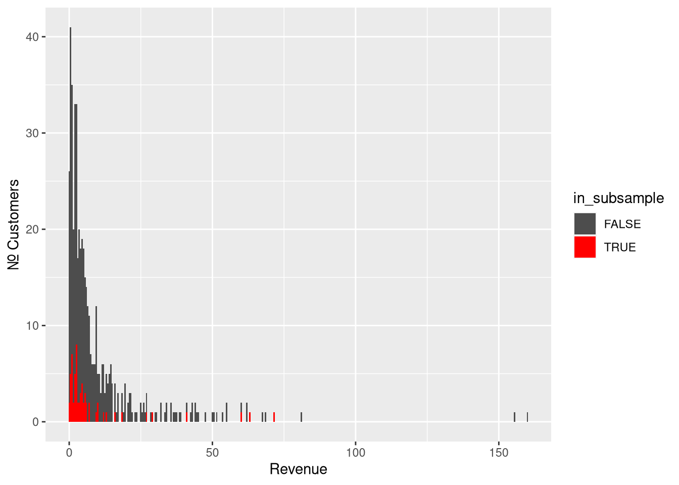
Figure 2: Subsampling 5% of the original sample
The subsample is a good representation of most of the distribution, but not
about the tail (which will appear much shorter than it really is). This is
not because we’re less likely to sample from any given customer in the tail.
It is because customers far out in the tail are simply more rare. A small sample
is not likely to carry any of them. For this particular sample and subsample:
| statistic | \(n\) | value |
|---|---|---|
| population mean (“true mean”) | \(\infty\) | 10 |
| sample mean | 500 | 9.71 |
| 5% subsample mean | 62 | 8.37 |
Fat Tail vs. Skinny Tail
We’ll explore the sampling behavior of our long-tailed distribution by comparing it to that of a skinny-tailed, exponential, distribution. The two distributions have same mean (10), and so the same total population revenue.
To make the distinction clear, I’ll refer to the long-tailed distribution as “fat-tailed” from here on.
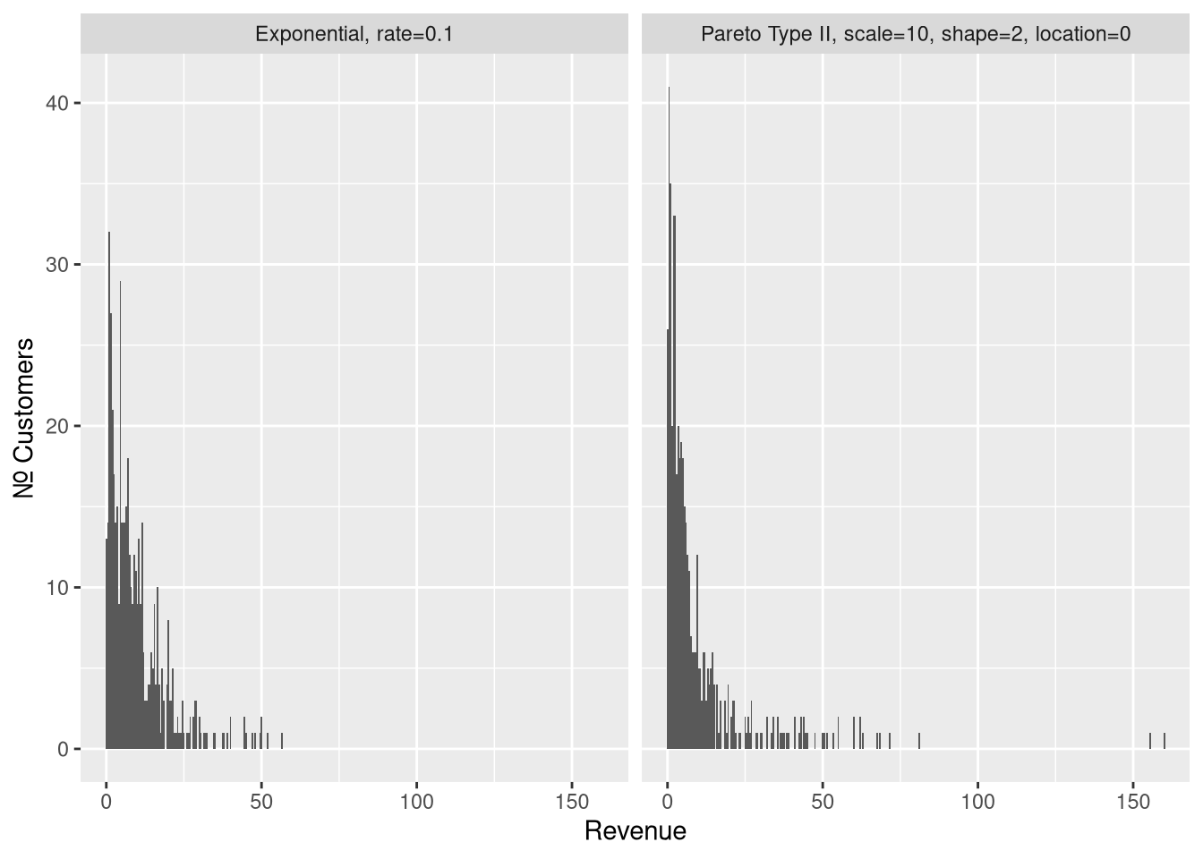
Figure 3: Samples (\(n = 500\)), from a skinny-tailed exponential on the left, and from our fat-tailed pareto distribution on the right.
These two are deceivingly similar. The Pareto distribution may very well be mistaken for a exponential distribution. What gives it away is the two samples at \(x > 150\). The probability of any single observation of \(x > 150\) is about \(\frac{1}{250}\) in our Pareto distribution, but less than \(\frac{1}{3,000,000}\) in the exponential distribution.
The difference in tail behavior is easier to see if we overlay the two cumulative distribution functions.
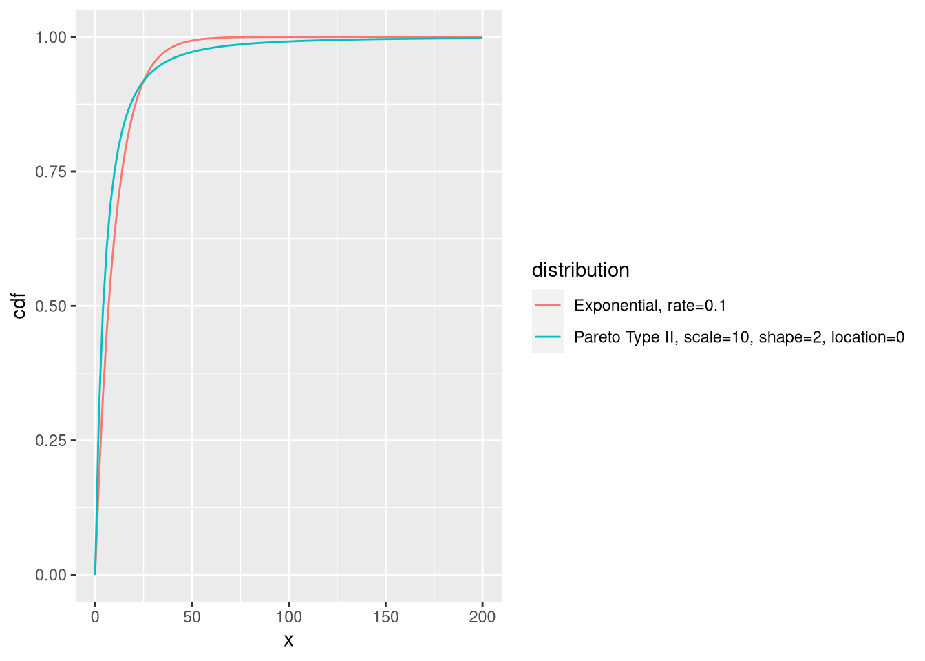
Figure 4: Cumulative Distribution Function of our Exponential and of our Pareto with mean = 10
The exponential distribution tapers off very quickly, and has virtually no mass beyond \(x > 75\). The Pareto distribution has some, and tapers off rather slowly. This makes observations beyond \(x > 150\) improbable enough to be rare, but plausible enough to happen from time to time.
Fat Tails and the Law of Large Numbers
The law of large numbers tells us that as \(n\) increases in a sample, the sample mean converges on the distribution mean. But… how fast? In simplest of terms: The fatter the tail, the slower, and more erratic will the convergence be.
- Slower: because the longer the tail, the more observations are required to properly sample it.
- More erratic: because each tail event will have a larger influence (a larger “jump”) on the sample mean.
If the distribution is sufficiently fat-tailed, (For example: Pareto distributions with shape \(\leq 1\)), it doesn’t even have a mean (think about what that means!), and there can be no convergence towards it.
This is bad news for us: Per-customer revenue distributions tend to have fairly fat tails, and will be slow to converge.
Below, we can see this in action: We’ll add one observation at a time to our sample, and see how our sample mean converges to the distribution mean.
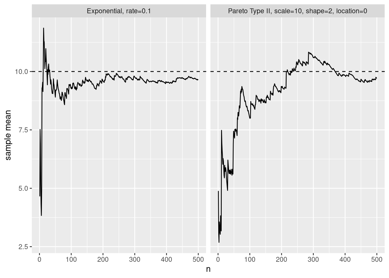
Figure 5: Variation of sample mean as more observations are added to the sample.
All examples we’ve seen now have been based on just one random sample & subsample. Let’s repeat the above experiment many (\(10^{4}\)) times to see what convergence towards the population mean looks like is on average.
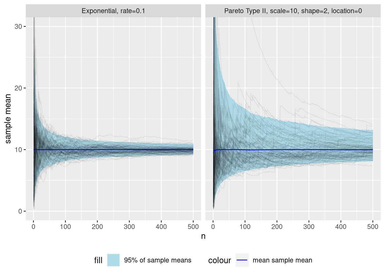
Figure 6: Distribution of sample mean as additional observations are added to the sample, across many simulations. To aid intuition, a subsample of 100 simulations are included as black lines with low opacity.
Whoa! Certainty about the sample mean increases much slower for the fat-tailed distribution. After \(n=50\) observations, we can be 95% confident its sample mean is within the interval \([7.4..13]\) for the exponential distribution. This might already be sufficient for useful inference. The Pareto distribution has a 95% interval of a whopping \([5.6..19]\).
Fast forward to \(n=500\), and the 95% interval for the Pareto distribution is still \([8.1..13]\). Meanwhile, the exponential distribution is at a respectable \([9.14..10.9]\).
Technical note: We’re usually interested in the reverse problem. That is: inferring a credible interval of the distribution mean from a sample. The level of uncertainty for that problem will be similar, but worse. (This is because tail shape parameter is unknown and difficult to estimate from data).
Okay, so the variance of the sampling distribution is huge… But hey, the mean sample mean (blue line) is bang on! So what was the fuzz about underestimating the mean?
Let’s take a closer look at the sample mean distribution at \(n = 30\) and \(n = 500\).
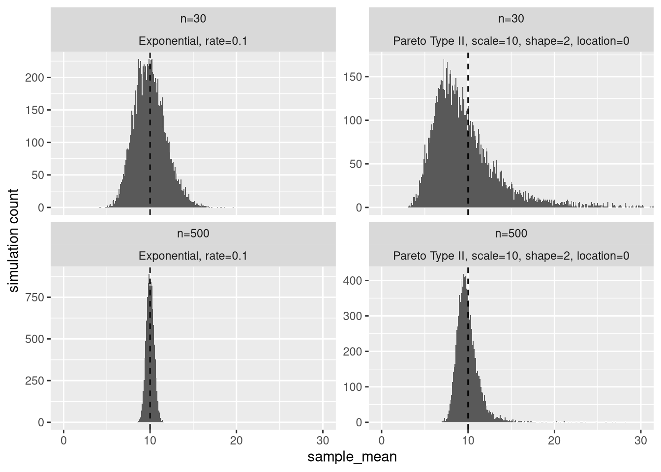
Figure 7: Distribution of sample mean at n=30 and n=500. The vertical dashed line is the distribution mean.
First, why did I choose \(n=30\)? Many statistics textbooks say that with 30 or more samples, the sampling distribution of the sample mean will be approximately Gaussian (Normal). This is thanks thanks to the Central Limit Theorem (CLT). Despite this, we see that the sampling distribution of the sample mean of our Pareto distribution has considerable skew. In fact, 64% of the distribution is below the distribution mean of 10. For the exponential distribution, this number is 53%.
Even at \(n=500\), the Pareto still has 59% of the sampling distribution below its mean. At that point, the exponential has since long (\(n \approx 100\)) settled within a percentage point of 50%.
Why skew matters
A hypothetical game
Let’s digress a bit more from our average revenue example. Let’s say you’re offered to play a lottery game. Entry into the game is costs 10 million USD, with a \(\frac{1}{10}\) chance of winning 200 million USD. (If you can’t pay the entry, let’s assume you’re given a one time credit).
The expected profit from this game is: \(\frac{1}{10} \times 200 - 10 = 10\) million USD.
Is it rational to play?
For most people, losing 10 million USD would amount to lifelong economic ruin. If that’s the case, even though the 10 million USD expected profit is unbiased, there’s a 90% risk of lifelong economic ruin.
What if you can afford to play several times, without risking ruin? Then since the expected profit is positive, it is probably rational to play.
Getting back to our example: If we try to estimate the distribution mean, from the sample mean, the average (this is what “expected” means) error (the dashed line in the histograms above), if we do it many times, is zero. But, if we only do it a single time: the most likely error is an underestimation (the peak of the distribution). For \(n=30\), we said 64% of the distribution is below sample mean. This percentage is how often you will underestimate the distribution mean if you do it naively from the sample mean.
Most business decisions are finite
Most business problems are somewhere in between these two extremes. You’ll be given a small to moderate (definitely not infinite) number of chances to let good decisions outweigh bad decisions. You are limited by:
The rate at which you can collect and analyze data
The rate at which new opportunities occur
Social norms and behavior. There’s only so many times you can change your mind about a proposal.
In a finite world, we must consider the entire distribution of outcomes – You might not make a sufficiently large number of decisions in order to have the rare large overestimation correct a large number of underestimations.
Business decisions usually have a truncating effect too – Since they are often binary, the sign (which alternative is better) of the error may be more important than the magnitude (by how much). This means we lose out on the effect of rare large overestimation canceling the effect of frequent small underestimations.
As an example of the truncating effect: Lets say you’re picking winners, based on average revenue, in a sequence of king-of-the-hill-style A/B tests. For some reason you consistently have a smaller sample size for the contender than the incumbent. Due to the sampling distribution skew, you will most often be biased in favor of the incumbent (which has less skew than the contender). If you’re doing this systematically, you have set yourself up to systematically make sub-optimal decisions.
So, what do we do?
The fundamental problem working with fat-tailed distribution is that the characteristics of the tail:
- Require a lot of samples to observe fully
- Have the largest impact on the characteristics of the distribution (for example mean and variance)
Short of changing your business model, there’s no way around this. (Log-transforming your data won’t work 🙃 – but it’s a good exercise to think about why it won’t help!).
Knowing to look for fat-tailed distributions
We won’t get our hands on with actual techniques for inference and quantifying uncertainty in this post.
Still, knowing to look for fat-tailed distributions goes a long way. We can be alert for when our statistical intuition might be off. In these cases, if you can’t afford a full probabilistic treatment – err on the high side with sample sizes.
Use pre-existing knowledge
One of the issues problems with fat-tailed distributions is that it’s difficult to estimate exactly how fat the tail is. (This is the shape-parameter in the Pareto distribution).
If your sample is small, you may not yet have observed a tail event. Your sample may then be indistinguishable from an exponential distribution.
If you have existing, similar data, you can reason about whether future tail events are likely (even though no events exist in your sample). You can even try to fit a distribution to your existing data to get an idea of how fat-tailed it is?
Use a hybrid of quantitative and qualitative reasoning
We have accepted that the tail is difficult to sample, and difficult to reason quantitatively about. Let’s instead focus on the lower part of the distribution. We can easily reason quantitatively about the non-tail, and try to reason about the tail qualitatively.
Let’s think about our business example.Even though the tail of our Pareto distributions contributes a disproportionately large amount of total revenue, the lower 98% still accounts for 82% of it. Also, the lower 98% is much easier to sample. (98% is arbitrarily chosen. Many variations of this exists. You might for example also choose to trim the bottom 1% and the top 1%, instead of the top 2%).
Qualitatively
Here’s the blank you have to fill in. You’ll need to use your judgment to reason about your top 2% customers. If you’re for example comparing customers from two competing channels, try to reason about their causal impact on your top 2% customers.
Quantitatively
Let’s look at simulations of the sample mean of the lower 98%.
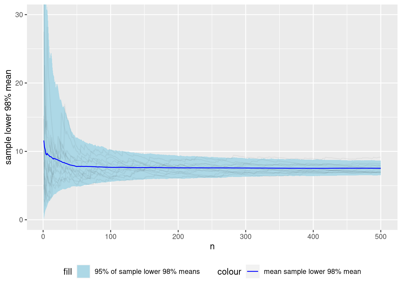
Figure 8: Distribution of sample lower 98% means of the Pareto distribution we’ve been using as a running example across many simulations.
As you can see, the sampling distribution of the lower 98% mean is much tamer than the “full” mean. At \(n = 50\), the 95% interval of the sample trimmed lower 98% mean is \([4.9..12.5]\). The 95% interval of the “full” mean was \([5.6..19]\).
Technical note: Below \(n=50\), the sampling distribution is biased, When \(n \times 0.98\) is non-integer, we weight the top (fractional) observation with \(w = n \times 0.98 - \lfloor n \times 0.98 \rfloor\). When \(n=50\), the most influential observation can finally be completely dropped. There are probably smarter ways to deal with the fractional observations which could remove this bias.
Note that we have not tackled any of the fundamental problems with the distribution. We have just changed focus to the part of the distribution that is less problematic.
Conclusion
This post became a bit of an bait-and switch. You were lured in with a particular business problem, but the perils of fat-tailed distributions are general. In fact, they probably apply to many, if not most of of your business metrics.
I hope to publish another post where we dig in a bit to inference techniques for this distribution.
Finally: The name of this post is of course inspired by Fooled by Randomness, by Nassim Nicholas Taleb. If you’re technically interested, I can recommend Statistical Consequences of Fat Tails, which is a companion text to his more popular books. It provides a great synopsis, is both approachable (compared to standard texts) and entertaining!